We discussed Fourier Series and how electromagnetic signals can be thought of as collections of frequency components. A filter is a circuit that attenuates signal components based on their frequencies. Filters are characterized by what range of frequencies they affect and by their order, which represents the degree of attenuation.
Frequency Ranges of Filters
| Low-Pass | Attenuates frequency components above a certain threshold |
| High-Pass | Attenuates frequency components below a certain threshold |
| Bandpass | Passes a contiguous range (band) of frequencies and attenuates frequencies outside that band |
| Band-Reject or Notch | Attenuates a band of frequencies |
Constructions of Filters
| Passive | Consist of passive components (resistors, capacitors, and inductors) |
| Active | Contain active components such as transistors and op amps. |
| Digital | Signals are digitized and processed as sets of digital values by logic circuitry or by firmware running on a processor. |
Passive Filters
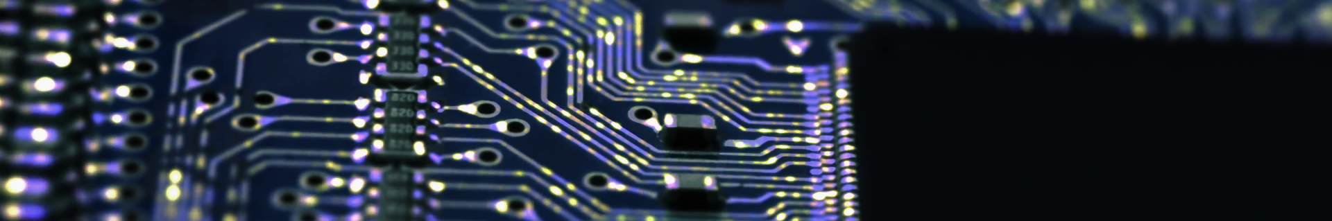
Passive filters consist of passive components: resistors, capacitors, and inductors. A quick way to determine what range of frequencies an arrangement of passive components will attenuate is to consider that capacitors act as short-circuits to high-frequency components and act as open-circuits to low-frequency components. Inductors are the opposite. And, resistors affect all frequency components equally. Check out the circuit below.
Passive Low-Pass Filter
The circuit has just one reactive component, the capacitor C1, and R1 and C1 form a voltage divider. By the voltage divider formula, Vout = Vin * ZC1/(ZR1+ZC1). So, the transfer function Vout/Vin is:

The capacitor C1 has high impedance to low-frequency components. So, at low frequency its impedance will be large resulting in the value of the transfer function being large. This means the filter passes low-frequency components. At high-frequency, the capacitor trends towards being a short circuit, so the value of the transfer function will be minimal at high frequency meaning the filter attenuates high-frequency components. This is a low-pass filter.
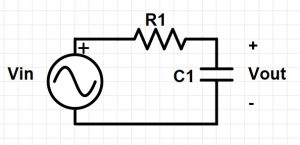
Now, let’s look in a bit more detail. The impedance of the capacitor is 1/sC, and the impedance of the resistor is R.
The transfer function, Vout/Vin, is then:

Note a couple things about this trasnfer function. First, it can not be greater than one, because resistance and capacitance of the components are positive numbers. When the transfer function has a value range of 1 or less, then it only attenuates and does not amplify. This will always be the case with passive filters, they only attenuate and their transfer functions always have a value less than 1.
Second, note that the numerator is a constant, and the denominator is a single order polynomial of s. This means that it is a 1st-order filter, since the order of a filter is the highest order of polynomial (highest power of s) in either the numerator or denominator of its transfer function. Transfer functions of circuits consisting of passive components will always be ratios of polynomials. This filter has no zeros and one pole at -1/RC, because that is the value of s that makes the denominator zero.
Filter Order: Highest polynomial order of transfer function numerator or denominator
As I said before, the poles and zeros of a circuit’s transfer function are key to the circuits behavior, and these values can be used as shortcuts for working with a circuit. The pole at -1/RC determines the threshold frequency beyond which this filter attenuates frequency components. That is to say it determines the cutoff frequency that is the dividing line between pass band and stop band. The cutoff frequency in radians is just the absolute value of the pole.
Cutoff Frequency: 
Low-Pass Filter AC Analysis
AC Analysis is analysis of the frequency response of the system, and this is a steady-state response of the system, not transitory. Mathematically, AC Analysis is concerned with the jω portion of the Laplace variable (s =σ + jω), not σ which is involved with the transient response. Substitute jω in for s in the transfer function to determine the Frequency Response. Then, convert to polar form to get magnitude and phase of the transfer function.
Frequency Response: Substitute jω for s in Transfer Function
In practice we use a computer tool to perform the AC Analysis. SPICE is a standardized circuit simulation platform, and there are a couple excellent free SPICE programs available. I highly recommend you install both of these and invest time to learn these tools thoroughly.
SPICE Programs:
- LT Spice: https://www.analog.com/en/design-center/design-tools-and-calculators/ltspice-simulator.html
- TINA-TI: http://www.ti.com/tool/TINA-TI
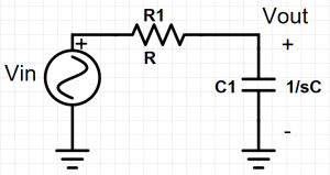
I will use LT Spice for low-pass filter analyses. AC Analysis in SPICE produces a graph of the frequency response of the transfer function showing its magnitude and phase. The scale may seem odd. The horizontal scale is logarithmic in decades (sub tics represent x1, x2, …, x9 and are not evenly spaced). The vertical scale for magnitude is also logarithmic, but it is in decibels (dB). Decibels for transfer functions involving voltage and/or current are 20•log(H(s)), where H(s) is the transfer function. Decibels for transfer functions involving power are 10•log(H(s)). The vertical scale for phase is linear and in units of degrees.
AC Analysis Horizontal Scale: Log scale in decades, Units: Hz.
AC Analysis Magnitude Vertical Scale: 20•log(H(s)), Units: dB.
AC Analysis Phase Vertical Scale: Linear Scale, Units: Degrees.
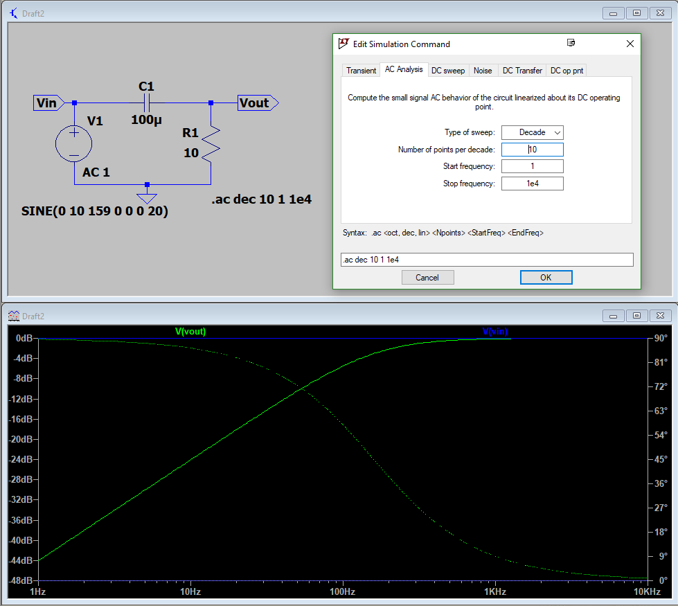
The dotted line is phase, and the solid line is magnitude. This low-pass filter has a 10 Ohm resistor and 100 uF capacitor, so the cutoff frequency is 1/(2*pi*R*C) = 159 Hz. Cutoff frequency is also called the 3dB frequency, because at that frequency, the magnitude is 3dB below maximum value (3dB = 1/sqrt(2) or .707). The cutoff frequency is somewhere between 100Hz on the graph and the next sub tic, and yes indeed, the magnitude does appear to be about -3dB there. And, the phase is -45 degrees at the cutoff frequency meaning the output waveform will be delayed by 45 degrees relative to the input.
At Low-Pass Filter Cutoff Frequency:
– Magnitude is 3 dB (or .707) below max.
– Phase is -45 degrees.
Let’s run a transient analysis to see what the output does in real time. I will configure the input voltage function as a sign wave with magnitude 10V and frequency 159 Hz (at the cutoff frequency).
There you have it. At the cutoff frequency, the output waveform magnitude is .707 times the input magnitude. And, the output phase is lagging input phase by 45 degrees. See how wonderful SPICE is?
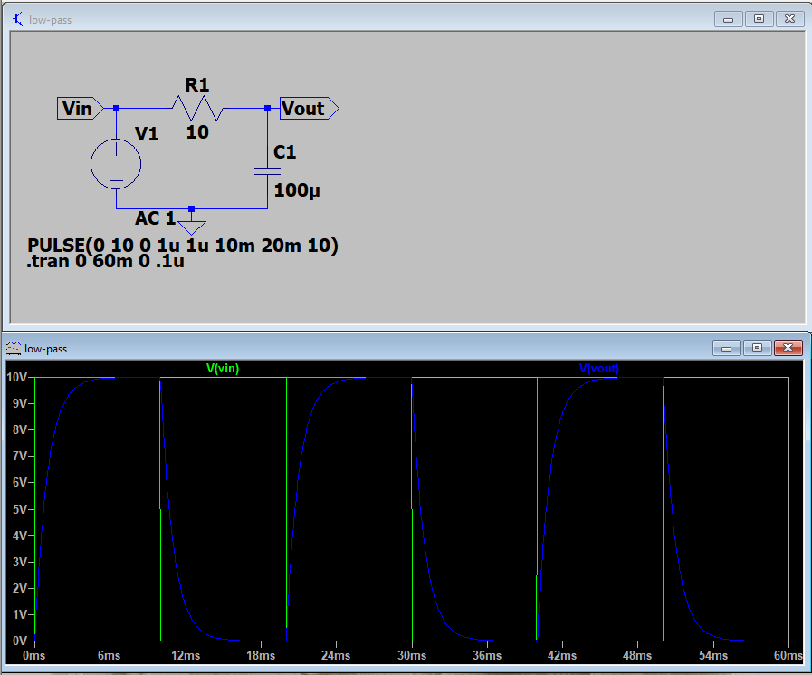
Low-Pass Effect on Square Wave
Below is a SPICE simulation showing the effect of a Low-Pass Filter on a square wave. The rising and falling edges of the output are slowed and approach their final values asymptotically (exponential decay).
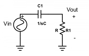
Passive High-Pass Filter
Now, let’s look at a high-pass filter, which passes high-frequency components and stops low-frequency components. If we swap positions of the resistor and the capacitor so that the capacitor is now in series with the signal we transform to a high-pass filter.
Transfer Function:

Based on the transfer function this is a first order filter, since there is no power of s higher than 1. Also, it has one zero at S = 0, and one pole at s = -1/RC. The cutoff frequency is determined by the pole, and therefore is the same as for the low-pass filter.
Cutoff Frequency = 
High-Pass Filter AC Analysis
AC Analysis with SPICE shows that the magnitude of the transfer function is low at low frequency, and increases until the cutoff frequency 1/(2*pi*RC) = 159 Hz where it levels out. As expected, the high-pass filter attenuates low-frequency signals and passes high-frequency signals.
High-Pass Filter Transient Analysis
Transient Analysis of the input set to a sine wave with frequency equal to the cutoff frequency yields an output whose phase precedes the input by 45 degrees (or lags by 315 degrees), and whose magnitude is .707 times input magnitude.