Oscilloscope measure voltage waveforms as functions of time. Current waveforms can also be measured using a current probe that measures current and outputs a proportional voltage (Hall Effect Sensor). The diagram below shows the fundamental design of an oscilloscope.
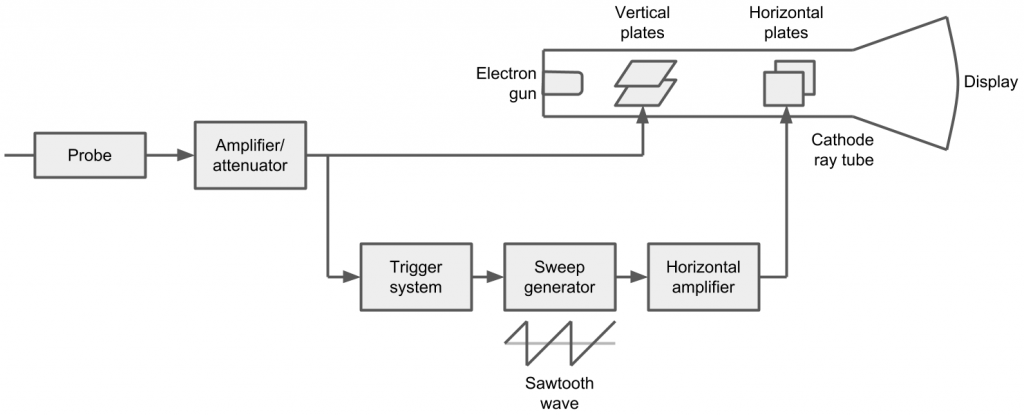
The basic idea is that an electron gun shoots a stream of electrons at the display, and the display illuminates where the electrons strike. Two sets of plates deflect the beam when voltage is applied to the plates, one deflects vertically and one horizontally. The horizontal deflection plates are driven by a saw-tooth wave that causes the illuminated point on the display to sweep from left to right, then jump back to the far left position, and then repeat. The vertical plates are driven by the measurement probe and cause the illuminated point on the display to move up or down as it sweeps across the screen. In this way an oscilloscope allows you to see the voltage waveform of a probed circuit node in real time.
Oscilloscopes also have trigger systems that wait for the probed signal to cross an adjustable voltage threshold before the sweep is triggered. The adjustable threshold is called the trigger level.
To give you an idea of how old I am, the first oscilloscope I used had a small convex screen made of a substance that would glow for some time after the electron beam hit it, so you can see a line tracing across the screen rather than a dot. And, one would connect a specialized Polaroid camera to the screen to capture your screenshot on film that would develop in a few minutes. Modern oscilloscopes digitize the measured signals using analog to digital converters and display waveforms on LCD screens. They also have USB or other I/O ports so you can capture and save screen shots.
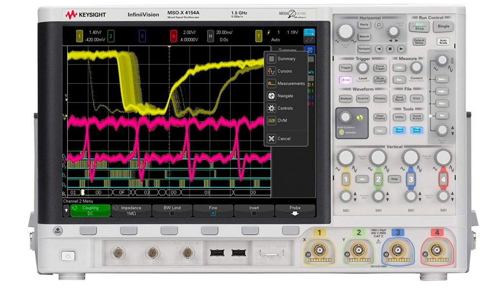
Let’s talk through the basic control on this Keysight scope.
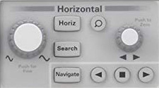
- Large knob scales the horizontal axis of the screen.
- Small knob slides the horizontal trigger position on the screen.
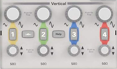
- Large knobs vertically scale the display of each waveform
- Small knobs vertically slide 0V line for each waveform
- Buttons turn on/off the display of each waveform
The 50Ohm indications below the vertical controls indicate the input impedance of each channel. They can be set to 50Ω, which is for a driver such as a function generator that expects to drive into a 50Ω load, or to high impedance (1MΩ) that is for probe measurements so as to not disturb the system under test.
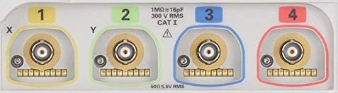
- Probe input channels – BNC Connectors
- Contacts below BNC are for communication between scope and probe
- Note the max input voltage warning of 300VRMS
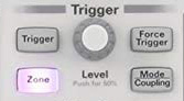
- Force Button triggers immediately
- Mode Button changes mode: Normal mode triggers only when trigger condition is met. Auto mode triggers constantly
- Knob adjusts the vertical level of the trigger threshold
- Trigger button selects type of trigger and channel source for trigger
Modern scopes have many different types of triggers:
- Trigger on a signal edge, either rising or falling, when its voltage crosses the trigger threshold.
- Trigger on a logic pattern of channel input voltages.
- Trigger on pulse width greater or smaller than
- Trigger on one channel OR another
- Trigger on certain patterns from a standard protocol
- Trigger on time threshold between edges of signal on two different channels (setup/hold time)
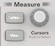
Measurements:
Max voltage, min V, avg V, RMS V, frequency, period, pulse high time, pulse low time, rise time, fall time, setup time, hold time, etc.
Scope Bandwidth
There is a limit to the frequency range that a scope can measure. It is determined by the scope bandwidth rating (1.5GHz for scope above), the sampling rate (5 GigaSamples/second above), and probe bandwidth and type. Scope bandwidth rating refers to the highest frequency component of a signal the scope can accurately measure. So, this scope can measure sine waves up to 1.5GHz, but square waves up to maybe only a tenth of 1.5GHz, since they have frequency components at 3rd, 5th, 7th, etc harmonic of the fundamental frequency of the square wave.
Probes
Careful attention to the probing solution is critical for accurate, trustworthy measurements. Different probe types have different trade-offs.
Passive Probes
Passive probes are less expensive than active probes, and they can handle much higher voltage. They consist just of conductors that bring the voltage of what you are probing up to the scope where it is received and measured. Because of this, they place more capacitance on the circuit under test than an active probe, which has an amplifier for the measurement right near the tip. And, passive probes add a large stub on transmission lines potentially causing massive reflections. Therefore, passive probes are for relatively low frequency digital and analog signals and for power signals that have high voltage.
Set scope input impedance to 1MΩ for all passive probes
An improvement for most measurements over the simple passive probe is represented by the 10:1 passive probe. The 10:1 probe adds a 9MOhm resistor in series, which from the point of view of the circuit under test increases its input impedance (Thevenin equivalent impedance) to 10MOhm and reduces the equivalent capacitance to something on the order of 15pF. The downside is that the scope now receives a voltage divided version of the signal being measured, and the division is 1/10th (1M/(1M + 9M)). So, the scope needs to detect the probe type as being 10:1 and scale the input accordingly, or the user needs to tell the scope that a 10:1 probe is being used.
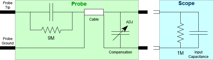
Many passive probes include an adjustment either at the end plugging into the scope or at the measurement tip end, or they have an internal adjustment that the scope adjusts automatically. The adjustment is for an adjustable capacitor that varies the frequency response to compensate for reactive parasitics in the probe. Scopes typically have an output connection point on the front that drives a square wave. Connect a probe to this, and make the adjustment to tune the measured square wave to have nice square corners. Remember from Fourier Analysis that those square corners are what contain the high-range frequency components, and tuning the waveform to be square indicates that your probe is tuned to pass the biggest range of frequency components with equal attenuation.

Passive probes are available in single-ended and in differential versions. Differential probes have two probe tips, and the difference of the two probed signals is measured. Single-ended probes measure a signal relative to ground and come with a ground lead or connection point. That ground connection is not isolated, it is connected to scope ground and AC earth ground. Do not connect the probe ground lead to a power line, it will short and maybe fry your probe.
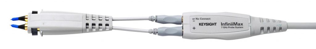
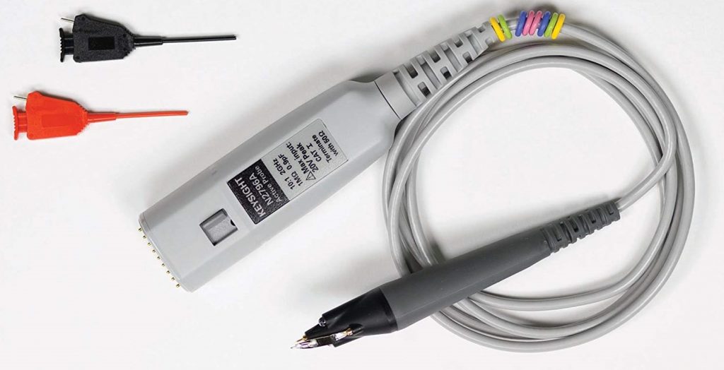
Active Probes
Active probes have an amplifier located near the tip. This allows them to place much less capacitance on the circuit under test, and they place a much smaller stub on transmission lines. They are the only solution for high frequency signals. Their downsides are expense and limited voltage range and expense. And, they are expensive.
Current Probes
Current probes are placed around a conductor, and a Hall Effect sensor measures the current flowing through the conductor and converts to a voltage waveform delivered to the scope.


Noise
It is a challenge to not pick up noise from electromagnetic interference. The two measurement leads for a differential probe, or the measurement lead and the ground lead of a single-ended probe form an antenna. The area of the antenna loop is proportional to how much EMI it will pick up. So, you need to minimize this area…use short leads. Or, sometimes you just need a crude look, and it is OK to use long leads, but be aware that some of the noise you see on the scope may not really be in the signal you are measuring.
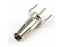
With passive probes, I rarely use the long ground lead that they come with. Instead I use probe sockets that can be soldered on to the measurement points, and these work really well to avoid picking up noise. They have signal and ground leads, and you can solder thin (30 gauge), short wires to the circuit under test to allow the connection to flex and not break.
Probe Setup
Before performing sensitive measurements, make sure you
Persistence
Persistence mode does not clear the screen after each sweep, but allows a configurable number of sweeps to build up and be displayed. This allows you to see where the waveform spends most of its time and also gives you an idea of how much it wanders and of rare events.

Eye Diagrams
Eye diagram measurements are used to see how much voltage and timing margin a signal has relative to a clock signal. They are so named because they resemble an eye. In Eye Diagram mode the scope turns on persistence, centers the trigger on the clock edge, and turns off the clock waveform, so just the data waveform is shown. The data waveform must meet minimum eye height, which is determined by VIH and VIL specs, and must meet minimum eye width, which is determined by TSU, TH and jitter specifications. Some signalling standards also have specifications for slew rate through the logic transition regions, which determines the slopes of the sides of the eye.

Here is a video from Keysight Labs discussing eye diagrams in more detail.
Next: Function Generators