
Gustav Kirchhoff was a German physicist who lived from 1824 to 1887, and he gave us two important laws for electric circuits. These are Kirchhoff’s Current Law and Kirchhoff’s Voltage Law, and they apply to all lumped element circuit models. Lumped element circuit models are as opposed to distributed element circuit models and basically mean circuit models that do not take into account the time it takes for electromagnetic waves to propagate over distance. Lumped element circuit models assume that changes in voltage and current happen at all elements in a circuit at the same time.
Electromagnetic waves propagate very quickly. In a vaccum, they move at the speed of light. In conductors on a circuit board, they move at something approaching the speed of light, something like 1/2 to 2/3 the speed of light. So, given this high speed, the lumped element circuit model assumption is a good one making Kirchoff’s laws very useful. It is only with very high frequency signals and/or long distances between elements that you need to move to a distributed element circuit model, which is also called transmission line theory.
I would like to mention that it is quick and easy to determine whether you need to use a distributed element model or a lumped element model, so the good news is that it is simple to determine when you need to worry about distributed element effects. We will cover this later, when we get to transmission line theory.
Kirchhoff’s Current Law (KCL)
Kirchhoff’s current law is quite simple and states that at any junction (AKA node) of a circuit, the sum of all the currents flowing into that junction is equal to the sum of all the currents flowing out of that junction. KCL applies when currents have reached steady state and when they are changing dynamically.
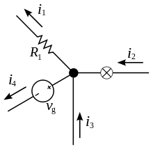

KCL: What goes in must come out
Think of KCL like the law of conservation of current: what goes in must come out.
Kirchoff’s Voltage Law (KVL)
Kirchoff’s voltage law states that all voltages around any closed path in a circuit sum to zero. As with KCL, KVL applies to steady state voltages and to dynamically changing voltages.
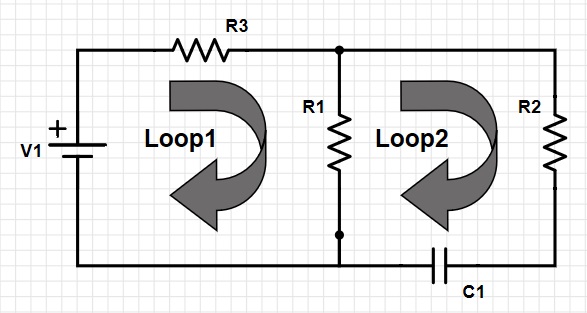
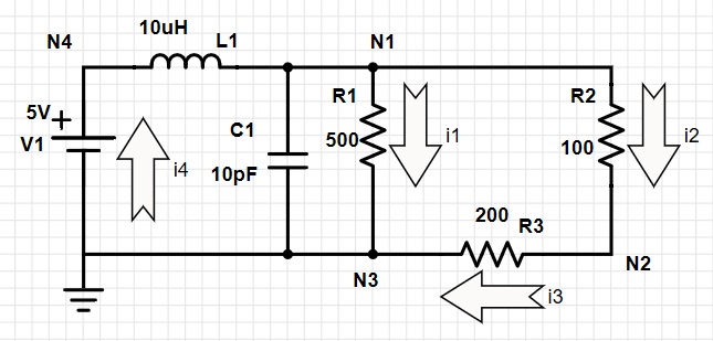
In the circuit above, the closed path labelled Loop1 consists of component V1, R3, and R1. By KVL, the sum of the voltages across these 3 components equals zero. For example, if voltage source V1 provides a 5V voltage increase, then the voltage drops across resistors R3 and R1 must sum to 5V. Closed path Loop2 consists of components R1, R2, and C1. The voltages across these components must also sum to zero. There is a 3rd closed path in the diagram above not labelled, and this consists of components V1, R3, R2, and C1. KVL also applies to the voltages across these components.
KVL: Voltages around any closed circuit path sum to zero
DC Circuit Analysis Using Kirchoff’s Laws
With KVL and KCL and with the relationship between voltage and current for each component, you can figure out the current through and the voltage across any and every element in a circuit. Let’s walk through an example, but let’s start with a simple example that has one DC voltage supply and several resistors. We will perform DC analysis in this example. The relationship between voltage and current for a resistor, remember, is Ohm’s Law, which is voltage across resistor equals current through resistor times resistance, V = I * R.
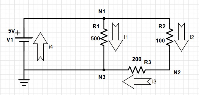
First of all, a note about signs and directions. In the circuit above, I have drawn arrows for current that point in the direction current flows. Current flows from – voltage to + voltage in a power supply, and flows from + voltage to – voltage in all passive components (resistors, capacitors, and inductors). With this arrow convention, current flowing in the direction of the arrow is positive, and current going against the arrow is negative. You could change this convention, flip everything around, and the math would still work fine, but NOBODY DOES THAT.
Regarding voltage convention for KVL, consider voltage rises as positive and voltage drops as negative. The voltage across the power supply is a rise, and the voltage across each passive component (resistor in this case) is a drop.
On with the analysis: Let’s write down all the equations we can for this circuit.
| KVL: | KCL: | Ohm’s Law: |
 |  |  |
 |  |  |
 |  |  |
We also know that node N3 is connected to ground (0V), because of the ground symbol on that node. So, since voltage supply V1 = 5V, the voltage at node N1 = 5V. OK, let’s take the 3rd KVL equation, substitute in Ohm’s law, and use KCL at N2, i2 = i3, to solve for i2.

i1 is easy to figure out from Ohm’s Law, since voltage at N1 and N3 are known: N1 = 5V, N3 = 0V. The voltage across R1, VR1 = VN1 – VN3 = 5V.

So, know we know i2, i3, and i1, which means we can calculate i4.

Great, we know all the currents. For the voltages, we know the voltage at nodes N1 (5V) and N3 (0V), so we just need N2. I think the easiest way is to calculate the voltage drop across R2 using Ohm’s law.
VR2 = 5/300 * 100 = 5/3 Volts. The voltage of N2 is then the voltage of N1 minus this drop.
Voltage of N2 = 5 – 5/3 = 10/3 Volts. We did it! All voltages and currents are known.
As you can see, even for this relatively simple circuit, it takes quite a bit of effort to perform the DC analysis by hand. So, in practice we would use a software tool to perform DC analysis for this circuit, because it would be faster and can provide nice pictures for our documentation. The software tools most often used for DC, AC, and transient analysis of lumped element circuits are called SPICE simulators.
DC and AC States of Capacitors and Inductors
To the circuit in the example above, let’s add an inductor and a capacitor and talk in high-level terms about how this affects AC and DC analysis.
For DC signals, which are signals that do not vary with time, an inductor acts like a short circuit (a low-impedance connection), and a capacitor acts like an open circuit. For high frequency AC signals, these components act in the opposite way: an inductor acts like an open circuit, and a capacitor acts like a short circuit. For signal frequencies that cause inductors and capacitors, depending on their values, to be somewhere in between a short and an open, things get interesting and complicated, and you have to perform the AC analysis to determine what voltage and current really do in the circuit.
High Frequency:
- Capacitor is Short Circuit
- Inductor is Open Circuit
Low Frequency:
- Capacitor is Open Circuit
- Inductor is Short Circuit
In the upgraded example circuit, then, the inductor and the capacitor actually have no effect on the DC analysis. The inductor acts as a short-circuit for the DC power supply…so like a wire. And, the capacitor acts like an open-circuit in parallel with R1 and the power supply…so like it was not connected at all. For AC analysis at high frequency and assuming we change the power supply to some AC function, the inductor is going to act like an open-circuit, so no signal is going to get past to the rest of the circuit…the rest of the circuit will all be pulled down to ground voltage. For AC analysis at some middle frequency, well, we need to learn some more stuff first, and on the job we will probably turn to computer tools such as SPICE simulators.