Superposition Principle
The Superposition Principle holds for the most part for electromagnetic signals, and it provides help with understanding and manipulating signals. The Superposition Principle in general form states that the total response at a particular place and time to two or more stimuli is the sum of the responses from each individual stimulus. For electrical engineers, this means that at a particular location, if there are signals present that are driven by mutliple sources, they add to create the resulting signal.
For exmple, if you drive a voltage sine wave of one amplitude and frequency onto a conductor, and you drive another voltage sine wave of a different amplitude and frequency onto that same conductor, what you would measure would be the sum of the two sine waves.
And, the Superposition Principle works in reverse too. You can use techniques to subtract out signals that you don’t care about, so you can see the signal(s) of interest. Also, you can implement circuits that modify just some of the components of a composite signal. For example, you can implement a low-pass filter that filters out just the high-frequency components of a signal. The Superposition Principle is you friend.
Think of any signal as a composite
Even when signals are not intentionally mixed, no signal is entirely clean in the practical world, always having some “noise” from a variety of sources. It is very helpful to think of any signal as a composite of component signals and that you can manipulate those components individually, at least to some extent. Imagine a high-speed memory data line. This carries the digital data signal, but also cross-talk from nearby signals, ground plane and power plane noise from driver and receiver, reflected signals from transmision line effects. All of these component signals can be addressed and minimized in different ways so that the receiver can reliably pick up the digital data signal out of that mess.
Fourier Analysis
Joseph Fourier was a French mathematician who lived from 1768 to 1830, and developed some mathematics that are very important for signal analysis and manipulation. He determined that pretty much any general function can be represented by sums of trigonometric functions, which are simpler and can be processed individually. He developed the Fourier Transform, which is an operation that decomposes a general function into trigonometric components, and the inverse Fourier Transform that synthesizes the components into a general function.
Any periodic function can be represented as a series of sinusoids
Specifically for periodic functions, Fourier showed us how to decompose any periodic function into a sum of a possibly infinite set of sine and cosine functions. This is called the Fourier Series. How on earth is decomposing one function into an inifinite series of functions helpful, you ask? Well, the really helpful thing about a fourier Series is that just the first few terms provide a good approximation of the general periodic function, and the more terms you calculate, the better your approximation with dimishing returns. So, you may only need to calculate the first 5 terms or so of the series, and you’ve got a really good approximation of the general function in a form that is easy to process.
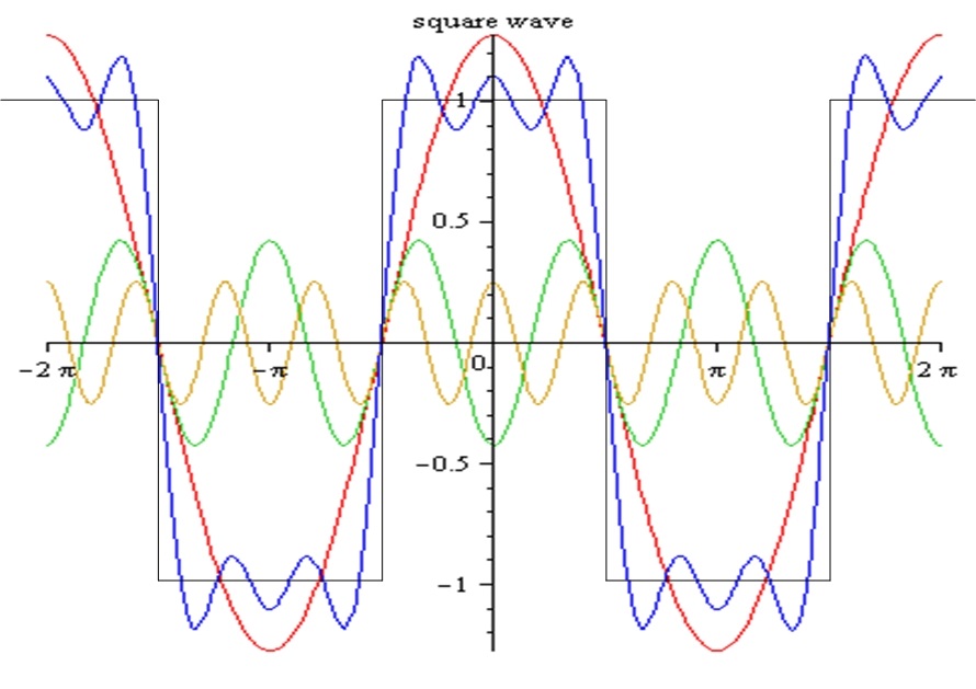
For example, imagine a square wave represented by a Fourier Series. The first term of the Fourier Series will be a sinusoid with same phase and frequency as the square wave. The next term will be a sinusoid of higher frequency (a harmonic, in fact) that when added to the 1st term results in a waveform that is more square. The 3rd term of the series will be a sinusoid of even higher frequency (higher order harmonic) that refines the waveform a bit more into a square shape, but has a lesser impact than the second term. There is no need to go on to infinity, because you get a pretty good approximation with the first few terms and can choose how good you want your approximation to be. In engineering, good approximations are what we deal with, not exactitudes. This Fourier Series approximation of a square wave is shown below. Red is the 1st term, green the 2nd, yellow the 3rd, and blue is the sum of these terms.
Digital signals are prevalent in modern electronics and are similar to square waves, so I want to point something out. From the preceeding discussion, you may have realized that the sharp corners of the square wave are what the higher frequency terms of the Fourier series deal with. In practice, when implementing a digital signal, you do not want those sharp corners, you want them nicely rounded, specifically because you do not want those higher frequency components. Higher frequency means more energy (according to Max Planck, and we should trust him, because he has an important constant named after him)…more energy to make and more energy carried, which radiated emissions standards frown upon. Also, those high-frequency radiated emissions have smaller wavelengths that can get out through smaller holes in your Faraday cage (I know I haven’t talked about Faraday cages yet, just bear with me). And, when you are talking about a voltage function, those sharp corners create more crosstalk, because that is where the highest rate of change of current is…Dang, really getting ahead of myself. The point is that those sharp corners have no benefit, and they cause problems, so avoid sharp corners in voltage waveforms in general.

By Lucas V. Barbosa – Own work, Public Domain, Link
Spectrum
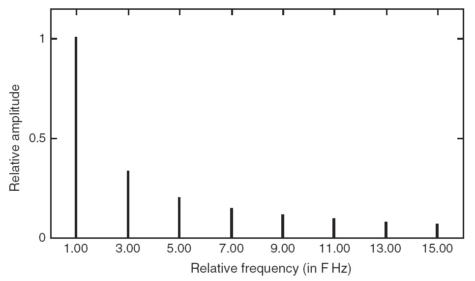
The Fourier Series representation of a signal is also referred to as that signal’s spectrum. Spectrum is the frequency-domain representation of a signal; it is the signal described in terms of frequency. You can think of spectrum as a graph of the signal with amplitude on the y-axis and frequency on the x-axis. The spectrum of a perfect, ideal square wave is shown in the graph below.
Spectrum is the representation of a signal in terms of frequency
Square waves in the real world are not perfect, and the spectrum does not consist of perfect straight lines at discrete frequencies. Instead, you tend to see Guassian distributions (bell curves) at discrete frequencies, like this:
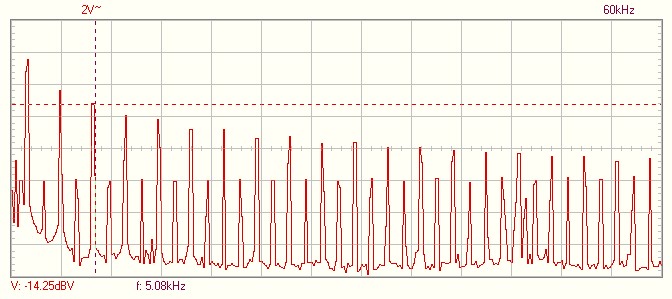
Thinking about signals in terms of their spectrums is important for a number of reasons. For example, if your design is going through radiated emissions regulatory testing, and you have a spectral peak that crosses the limit at 900MHz, and you see peaks at 300MHz, 900MHz, and 1.5GHz, you might think, “Oh crap, my memory clock is a 300MHz square wave. Well, at least I know the source of the failure.” Also, spectral thinking helps you realize how to process and manipulate signals. Want to turn a square wave into a sine wave? Easy peasy, just implement a frequency filter that passes frequencies at or below the frequency of the square wave, and blocks frequncies above that of the square wave. Want to mathemtaically shift the frequency of a square wave? Perform a fourier transform and get the 1st five or so terms of the Fourier Series, change the frequency of the 1st term to the new frequency you want, and change the other terms to be appropriate harmonics of that new frequency. Then, inverse Fourier transform that puppy, and you have achieved your desire.
I have to disclose something. Manually performing Fourier transforms and their inverses is complex and tedious. There’s calculus, complex number exponentials, and it really sucks. You may have noticed that I did not go into the actual math involved with these things, and I certainly don’t remember how to do it 20 years out of college. But, thankfully, we have excellent computer tools that can do this stuff for us. Heck, even oscilloscopes usually have a function called FFT (fast Fourier transform) that will show you the spectrum of a signal you are measuring with the click of a mouse. EEs do not do Fourier analysis manually unless for a very specialized reason, but it is important to understand what it is and how it can be used.
Below is a video discussing Fourier and Laplace Transformations by Brian Douglas. Excellent video!
Next: Resistors