
The Transfer Function of a circuit is defined as the ratio of the output signal to the input signal in the frequency domain, and it applies only to linear time-invariant systems. It is a key descriptor of a circuit, and for a complex circuit the overall transfer function can be relatively easily determined from the transfer functions of its subcircuits. Transfer functions are typically denoted with H(s).
Transfer Function H(s) = Output Signal / Input Signal
In circuit boards, unless you are using wireless technology, signals are voltage or current. A circuit’s input signal may be current or voltage and its output may be either as well. This creates four types of transfer functions that we have names for.
| Transfer Type | Output / Input | Units |
| Transadmittance H(s) | I(s) / V(s) | 1/Ω |
| Voltage H(s) | V(s) / V(s) | Unitless |
| Current H(s) | I(s) / I(s) | Unitless |
| Transimpedance H(s) | V(s) / I(s) | Ω |
Using Transfer Functions
Now, I would like to show you how to use the transfer functions of subcircuits to determine the overall transfer function of an electronic system. We will do this at a high level and not yet down at the level of individual circuit components.
Series and Parallel Combinations
If two subcircuits are connected in series, then the overall transfer function is the product of the transfer functions of the subcircuits. If two subcircuits are connected in parallel, and their outputs are summed, then the overall transfer function is the sum of the transfer functions of the subcircuits.
Series Connection of Transfer Functions

Parallel Connection of Transfer Functions

Let’s do an example. Here is a circuit that has two subcircuits in parallel with a 3rd subcircuit. What is the overall transfer function?
The series elements multiply to make: H1(s) * H2(s). This is then in parallel with H3(s). So, the overall transfer function is:
H(s) = Y(s) / X(s) = H1(s) * H2(s) + H3(s)
Feedback Transfer Function
The diagram below shows a feedback control system with G(s) forward gain, and H(s) feedback transfer function. E(s) is the error signal, which is the difference between the input signal X(s) and the feedback signal H(s)Y(s).


The overall transfer function of a feedback system, which is sometimes called the closed-loop transfer function, is the [forward gain] / (1 + [open-loop gain])
Open-Loop Gain: 
Closed Loop Transfer Function: 
Poles and Zeros
Transfer functions for circuits have the form of a ratio of polynomials of s. Polynomials can be factored to create a factored form of the transfer function.
| Polynomial Form: |  |
| Factored Form: |  |
K is a constant. Each of the values of s that results in the numerator being zero are called ZEROS. These are apparent in the factored form. And, each value of s that results in the denominator being zero is called a pole. The reason for the term ‘pole’, is that the transfer function’s value shoots up or down to infinity when s equals one of these values. The poles and zeros of a transfer function are used to determine a number of characteristics of circuits such as stability and responsiveness of a feedback control system. We will be talking alot more about poles and zeros in the future.
Complex Number Formats
The Laplace variable s is a complex variable and so poles and zeros are complex numbers. I would like to interject a quick discussion of complex number formats, because EEs use complex numbers alot and need to be able to easily convert between representations for the task at hand. Complex numbers are two-dimensional numbers. They have a real part and an imaginary part, and they can be represented in rectangular form or in polar form. Let’s graph a complex number represented by a dot on the complex number plane.
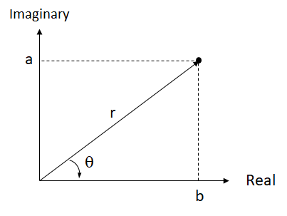
The value of the dot can be described in rectangular form as a + bj where a is the real part and b is the imaginary part. Or, it can be described in polar form as r ∠ θ where r is the magnitude of the vector from the origin to the complex value and θ is the angle of that vector relative to the real axis.
Rectangular Form: a + bj
Polar Form: r ∠ θ
Convert from Polar to Rectangular
To convert from polar form to rectangular form, we will use some simple trigonometry. Remember the famous mnemonic: SOH-CAH-TOA. Sine is opposite over hypotenuse, cosine is adjacent over hypotenuse, and tangent is opposite over adjacent.
b = r * cos (θ)
a = r * sin (θ)
Convert from Rectangular to Polar
To convert from rectangular to polar form, we will use tan(θ) = a/b and Pythagoras’ Theorum.
θ = arctan (a/b)
r = √(a2 +b2)
Helpful Videos:
I have to to do some editorializing. The technique of this guy, Mr. Brunton, below is amazing. Not only does he shun the blackboard behind him for the more techy glass surface in between him and the camera. But, while you are wondering if this is a new episode of CSI, you realize that he is writing those rather complex equations in mirror-image. And, his handwriting is still better than any professor I had! That is some serious badassitude right there. And, he’s got the TED talk shirt on…totally nailed it.